viziphant.gpfa.plot_trajectories

viziphant.gpfa.plot_trajectories(returned_data, gpfa_instance, dimensions=[0, 1], block_with_cut_trials=None, neo_event_dict={}, orthonormalized_dimensions=True, trials_to_plot=array([0, 1, 2, 3, 4, 5, 6, 7, 8, 9, 10, 11, 12, 13, 14, 15, 16, 17, 18, 19]), trial_grouping_dict=None, colors='grey', markers=('.', 'o', 'v', '^', '<', '>', '8', 's', 'p', '*', 'h', 'H', 'D', 'd', 'P', 'X'), plot_group_averages=False, plot_args_single={'alpha': 0.4, 'linestyle': '-', 'linewidth': 0.3}, plot_args_marker={'alpha': 0.4, 'markersize': 5}, plot_args_average={'alpha': 1, 'linestyle': 'dashdot', 'linewidth': 2}, plot_args_marker_start={'label': 'start', 'marker': 'p', 'markersize': 10}, figure_kwargs={}, verbose=False)

This function allows for 2D and 3D visualization of the latent space variables identified by the GPFA.

Optional visual aids are offered such as grouping the trials and color coding their traces. Changes to optics of the plot can be applied by providing respective dictionaries.

This function is an adaption of the MATLAB implementation by Byron Yu which was published with his paper: (Yu et al., 2009)

Parameters:

returned_datanp.ndarray or dict

When the length of returned_data is one, a single np.ndarray, containing the requested data (the first entry in returned_data keys list), is returned. Otherwise, a dict of multiple np.ndarrays with the keys identical to the data names in returned_data is returned.

N-th entry of each np.ndarray is a np.ndarray of the following shape, specific to each data type, containing the corresponding data for the n-th trial:

latent_variable_orth: (#latent_vars, #bins) np.ndarray

latent_variable: (#latent_vars, #bins) np.ndarray

y: (#units, #bins) np.ndarray

Vsm: (#latent_vars, #latent_vars, #bins) np.ndarray

VsmGP: (#bins, #bins, #latent_vars) np.ndarray

Note that the num. of bins (#bins) can vary across trials, reflecting the trial durations in the given spiketrains data.

gpfa_instanceGPFA

Instance of the GPFA() class in elephant, which was used to obtain returned_data.

dimensionslist of int, optional

List specifying the indices of the dimensions to use for the 2D or 3D plot. Default: [0, 1]

block_with_cut_trialsneo.Block or None, optional

The neo.Block should contain each single trial as a separate neo.Segment including the neo.Event with a specified neo_event_name. Default: None

neo_event_dictdict, optional

Dictionary of names and properties of the events that should be plotted onto each trajectory. The key specifies the label appearing in the legend. The item specifies the neo_event_properties, which are used by neo.utils.get_events() to filter the event. In case more than one event per dict-entry is available, only the first one is chosen to be plotted. Please specify more properties to narrow down the choice in that case. Default: {}

orthonormalized_dimensionsbool, optional

Boolean which specifies whether to plot the orthonormalized latent state space dimension corresponding to the entry ‘latent_variable_orth’ in returned data (True) or the unconstrained dimension corresponding to the entry ‘latent_variable’ (False). Beware that the unconstrained state space dimensions ‘latent_variable’ are not ordered by their explained variance. These dimensions each represent one Gaussian process timescale $ au$. On the contrary, the orthonormalized dimensions ‘latent_variable_orth’ are ordered by decreasing explained variance, allowing a similar intuitive interpretation to the dimensions obtained in a PCA. Due to the orthonormalization, these dimensions reflect mixtures of timescales. Default: True

trials_to_plotstr, int, list or np.array(), optional

Variable that specifies the trials for which the single trajectories should be plotted. Can be a string specifying ‘all’, an integer specifying the first X trials or a list specifying the trial ids. Internally this is translated into a np.array() over which the function loops. Default: np.arange(20)

trial_grouping_dictdict or None, optional

Dictionary which specifies the groups of trials which belong together (e.g. due to same trial type). Each item specifies one group: its key defines the group name (which appears in the legend) and the corresponding value is a list or np.ndarray of trial IDs. Default: None

colorsstr or list of str, optional

List of strings specifying the colors of the different trial groups. The length of this list should correspond to the number of items in trial_grouping_dict. In case a string is given, all trials will share the same color unless trial_grouping_dict is specified, in which case colors will be set automatically to correspond to individual groups. Default: ‘grey’

markerslist of str, optional

List of strings specifying the markers of the different events. Default: Line2D.filled_markers

plot_group_averagesbool, optional

If True, trajectories of those trials belonging together specified in the trial_grouping_dict are averaged and plotted. Default: False

plot_args_singledict, optional

Arguments dictionary passed to ax.plot() of the single trajectories.

plot_args_markerdict, optional

Arguments dictionary passed to ax.plot() for the single trial events.

plot_args_averagedict, optional

Arguments dictionary passed to ax.plot() of the average trajectories. if ax is None.

plot_args_marker_startdict, optional

Arguments dictionary passed to ax.plot() for the marker of the average trajectory start.

figure_kwargsdict, optional

Arguments dictionary passed to plt.figure(). Default: {}

verbose: bool

Print hopefully helpful messages for debugging purposes. Default: False

Returns:

figmatplotlib.figure.Figure

axesmatplotlib.axes.Axes

Examples

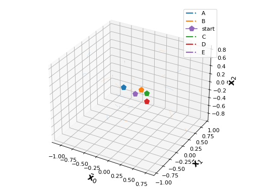
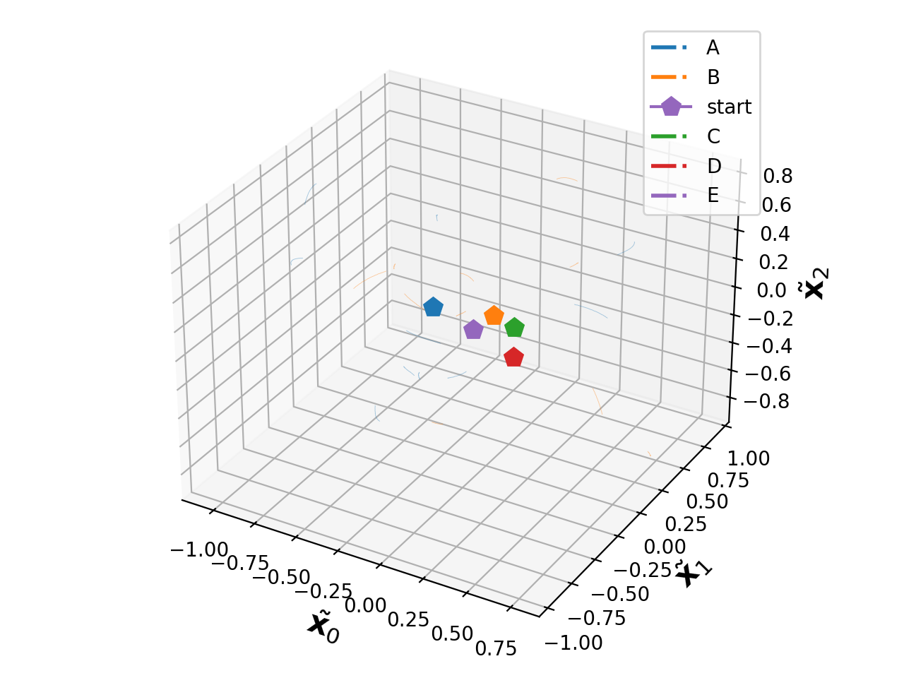
In the following example, we calculate the neural trajectories of 20 independent Poisson spike trains recorded in 50 trials with randomized rates up to 100 Hz and plot the resulting orthonormalized latent state space dimensions.

import numpy as np
import quantities as pq
from elephant.gpfa import GPFA
from elephant.spike_train_generation import StationaryPoissonProcess
from viziphant.gpfa import plot_trajectories
from matplotlib import pyplot as plt

data = []
for trial in range(50):
    n_channels = 20
    firing_rates = np.random.randint(low=1, high=100,
                                     size=n_channels) * pq.Hz
    spike_times = [StationaryPoissonProcess(rate=rate
                                            ).generate_spiketrain()
                   for rate in firing_rates]
    data.append(spike_times)

gpfa = GPFA(bin_size=20*pq.ms, x_dim=8)
gpfa.fit(data)

results = gpfa.transform(data, returned_data=['latent_variable_orth',
                                              'latent_variable'])

trial_id_lists = np.arange(50).reshape(5, 10)
trial_group_names = ['A', 'B', 'C', 'D', 'E']

trial_grouping_dict = {}
for trial_group_name, trial_id_list in zip(trial_group_names,
                                           trial_id_lists):
    trial_grouping_dict[trial_group_name] = trial_id_list

plot_trajectories(results,
                  gpfa,
                  dimensions=[0, 1, 2],
                  trial_grouping_dict=trial_grouping_dict,
                  plot_group_averages=True)
plt.show()

(Source code, png, hires.png, pdf)