viziphant.rasterplot.rasterplot_rates

viziphant.rasterplot.rasterplot_rates(spiketrains, key_list=[], groupingdepth=0, spacing=[8, 3], colorkey=0, pophist_mode='color', pophistbins=100, right_histogram=<function mean_firing_rate>, righthist_barwidth=1.01, filter_function=None, histscale=0.1, labelkey=None, markerargs={'marker': '.', 'markersize': 4}, separatorargs=[{'color': '0.8', 'linestyle': '--', 'linewidth': 2}, {'color': '0.8', 'linestyle': '--', 'linewidth': 1}], legend=False, legendargs={'handletextpad': 0, 'loc': (0.98, 1.0), 'markerscale': 1.5}, ax=None, style='ticks', palette=None, context=None)

This function plots the dot display of spike trains alongside its population histogram and the mean firing rate (or a custom function).

Optional visual aids are offered such as sorting, grouping and color coding on the basis of the arrangement in list of spike trains and spike train annotations. Changes to optics of the dot marker, the separators and the legend can be applied by providing a dict with the respective parameters. Changes and additions to the dot display itself or the two histograms are best realized by using the returned axis handles.

Parameters:

spiketrains: list of neo.SpikeTrain or list of list of neo.SpikeTrain

List can either contain Neo SpikeTrains object or lists of Neo SpikeTrains objects.

key_list: str or list of str

Annotation key(s) for which the spike trains should be ordered. When list of keys is given the spike trains are ordered successively for the keys. By default the ordering by the given lists of spike trains have priority. This can be bypassed by using an empty string ‘’ as list-key at any position in the key_list.

groupingdepth: int

• 0: No grouping (default)

• 1: grouping by first key in key_list.

  Note that when list of lists of spike trains are given the first key is by the list identification key ‘’. If this is unwanted the empty string ‘’ can be placed at a different position in key_list.

• 2: additional grouping by second key respectively

The groups are separated by whitespace specified in the spacing parameter and optionally by a line specified by the the separatorargs.

spacing: int or list of int

Size of whitespace separating the groups in units of spike trains. When groupingdepth == 2 a list of two values can specify the distance between the groups in level 1 and level 2. When only one value is given level 2 spacing is set to half the spacing of level 1. Default: [5, 3]

colorkey: str or int (default 0)

Contrasts values of a key by color. The key can be defined by its namestring or its position in key_list. Note that position 0 points to the list identification key (‘’) when list of lists of spike trains are given, if not otherwise specified in key_list!

pophist_mode: str

• total: One population histogram for all drawn spike trains

• color: Additionally to the total population histogram,

  a histogram for each colored subset is drawn (see colorkey).

pophistbins: int (default 100)

Number of bins used for the population histogram.

right_histogram: function

The function gets ONE neo.SpikeTrain object as argument and has to return a scalar. For example the functions in the elephant.statistics module can be used. (default: mean_firing_rate) When a function is applied is is recommended to set the axis label accordingly by using the axis handle returned by the function: axhisty.set_xlabel(‘Label Name’)

righthist_barwidth: float (default 1.01)

The bin width of the right side histogram.

filter_function: function

The function gets ONE neo.SpikeTrain object as argument and if the return is True the spike train is included; if False it is exluded.

histscale: float (default .1)

Portion of the figure used for the histograms on the right and upper side.

labelkey: int or string or None

• 0, 1: Set label according to first or second key in key_list.

  Note that the first key is by default the list identification key (‘’) when list of lists of spike trains are given.

• ‘0+1’: Two level labeling of 0 and 1

• annotation-key: Labeling each spike train with its value for given

  key

• None: No labeling

Note that only groups (-> see groupingdepth) can be labeled as bulks. Alternatively you can color for an annotation key and show a legend.

markerargs: dict

Arguments dictionary is passed on to matplotlib.pyplot.plot()

separatorargs: dict or list of dict or None

If only one dict is given and groupingdepth == 2 the arguments are applied to the separator of both level. Otherwise the arguments are of separatorargs[0] are applied to the level 1 and [1] to level 2. Arguments dictionary is passed on to matplotlib.pyplot.plot() To turn of separators set it to None.

legend: bool

Show legend?

legendargs: dict

Arguments dictionary is passed on to matplotlib.pyplot.legend()

ax: matplotlib axis or None (default)

The axis onto which to plot. If None a new figure is created. When an axis is given, the function can’t handle the figure settings. Therefore it is recommended to call seaborn.set() with your preferred settings before creating your matplotlib figure in order to control your plotting layout.

style: str

seaborn style setting. Default: ‘ticks’

palette: str or sequence

Define the color palette either by its name or use a custom palette in a sequence of the form ([r,g,b],[r,g,b],…).

context: str

‘paper’(default) | ‘talk’ | ‘poster’ seaborn context setting which controls the scaling of labels. For the three options the parameters are scaled by .8, 1.3, and 1.6 respectively.

Returns:

axmatplotlib.axes.Axes

The handle of the dot display plot.

axhistxmatplotlib.axes.Axes

The handle of the histogram plot above the the dot display

axhistymatplotlib.axes.Axes

The handle of the histogram plot on the right hand side

See also

rasterplot

simplified raster plot

eventplot

plot spike times in vertical stripes

Examples

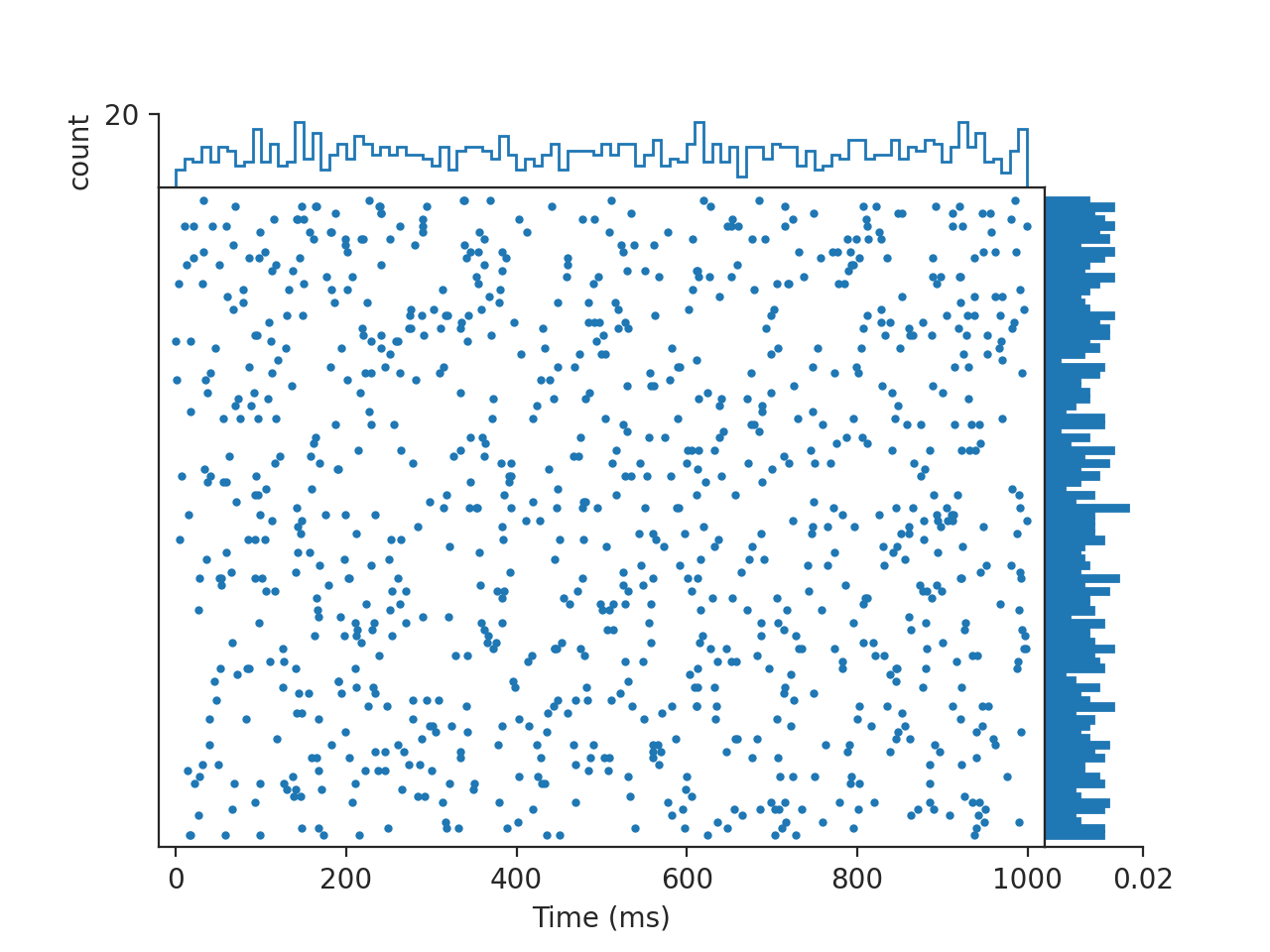
1. Basic Example.

from elephant.spike_train_generation import             homogeneous_poisson_process, homogeneous_gamma_process
import quantities as pq
import matplotlib.pyplot as plt
from viziphant.rasterplot import rasterplot_rates

spiketrains = [homogeneous_poisson_process(rate=10 * pq.Hz)
               for _ in range(100)]
rasterplot_rates(spiketrains)
plt.show()

(Source code, png, hires.png, pdf)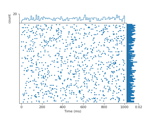

2. Plot visually separated realizations of different neurons.

from elephant.spike_train_generation import             homogeneous_poisson_process, homogeneous_gamma_process
import quantities as pq
import matplotlib.pyplot as plt
from viziphant.rasterplot import rasterplot_rates

spiketrains1 = [homogeneous_poisson_process(rate=10 * pq.Hz)
                for _ in range(100)]
spiketrains2 = [homogeneous_gamma_process(a=3, b=10 * pq.Hz)
                for _ in range(100)]
rasterplot_rates([spiketrains1, spiketrains2])
plt.show()

(Source code, png, hires.png, pdf)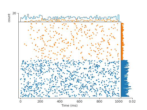

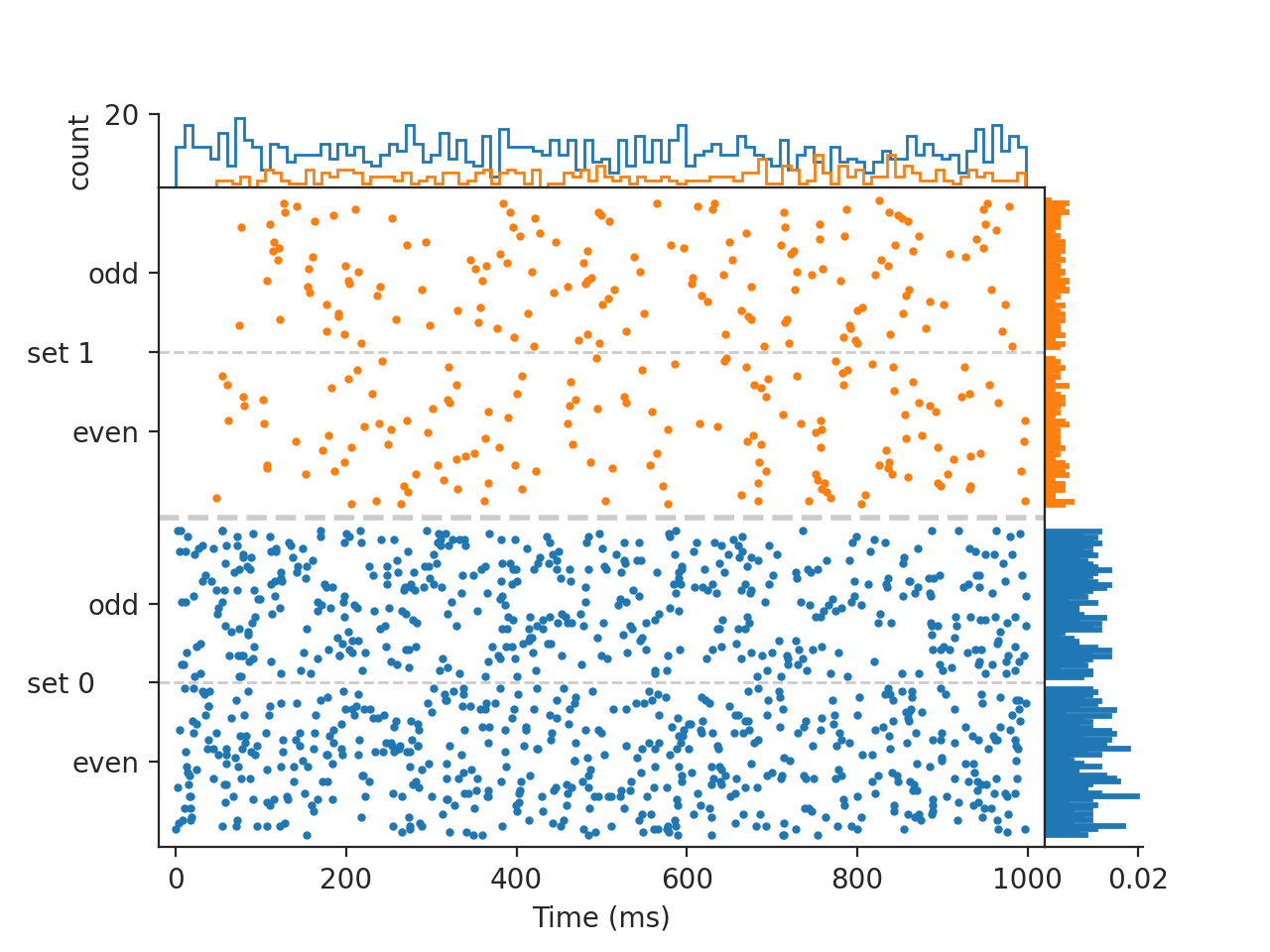
3. Add annotations to spike trains.

from elephant.spike_train_generation import             homogeneous_poisson_process, homogeneous_gamma_process
import quantities as pq
import matplotlib.pyplot as plt
from viziphant.rasterplot import rasterplot_rates

spiketrains1 = [homogeneous_poisson_process(rate=10 * pq.Hz)
                for _ in range(100)]
spiketrains2 = [homogeneous_gamma_process(a=3, b=10 * pq.Hz)
                for _ in range(100)]
for i, (st1, st2) in enumerate(zip(spiketrains1, spiketrains2)):
    if i % 2 == 1:
        st1.annotations['parity'] = 'odd'
        st2.annotations['parity'] = 'odd'
    else:
        st1.annotations['parity'] = 'even'
        st2.annotations['parity'] = 'even'

# plot separates the lists and the annotation values within each list
rasterplot_rates([spiketrains1, spiketrains2], key_list=['parity'],
                  groupingdepth=2, labelkey='0+1')

(Source code, png, hires.png, pdf)

'' key change the priority of the list grouping:

rasterplot_rates([spiketrains1, spiketrains2],
                  key_list=['parity', ''],
                  groupingdepth=2, labelkey='0+1')

Groups can also be emphasized by an explicit color mode:

rasterplot_rates([spiketrains1, spiketrains2],
                  key_list=['', 'parity'],
                  groupingdepth=1, labelkey=0, colorkey='parity',
                  legend=True)